Array Plot: 3D-Plot or XY-Plot of Array Data

This command allows a 3D-Plot or a XY-Plot of scalar values that are given in a matrix of m lines and n columns (see image and demo “arrayview.dem”).

Following dialog shows the available options:

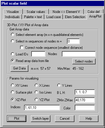
Get Array Data

Select element array (m x n quadrilateral elements)

Using this option an area of m x n quadrilateral elements has to be selected in an element selection dialog. If body elements are contained in the selection, only those surfaces of them are used, of which the corner nodes are contained in the current node selection, that means, with body elements also a node selection must first be done and stored. The border of the selected element area is determined and graphically displayed. The 4 corner nodes of the selected 4 sided area are also marked by a symbol then the 2 corners of the edge, that is to be used as x axis in the plot must graphically be selected. The given scalar values at the corner nodes of the selected elements are stored in a matrix to be plotted.

Select m sequences of nodes

This option allows plotting the given scalar values at the nodes of 1 or more sequences of nodes (lines) in one XY Plot. The sequences of nodes have to be selected graphically, where each sequence has the same number (n) of nodes. The number (m) of sequences must be given in the input field. The scalar values in the selected nodes are then stored as array data in a (m/n) matrix, where each node sequence defines one line of the matrix. The selected nodes are ordered in the sequence they are selected, when selected by a single point selection, if selected by giving a rectangle or polygon area, they are ordered in the sequence of their internal node ID. If the option „Correct node sequence“ is marked, the nodes are newly ordered so that the distance of pursuing nodes is smallest. The lines are immediately plotted after selection.

Load IDs

This option can be used, if several load cases of node or element related scalar values are given. In the input field, the smallest and the largest ID of load cases to be used must be given. Additionally the nodes (elements) for which a XY-Plot of the data should be done have to be given in the input field (internal IDs). A continuous area may be given in the form k1,-k2,kd where k1 is the smallest, k2 the largest ID and kd the increment. Clicking button “Select graphically”, the nodes (elements) can be selected graphically. For each node (element) a matrix line is provided, that contains the scalar values of the node (element) given for the sequence of load cases. The number of array lines corresponds to the number of selected nodes (elements) and the length of the lines corresponds to the number of given load cases. This option is useful when the load cases correspond to time steps of an incremental calculation (data types 8 or 9), and the time dependent curves for several nodes (elements) should be plotted in a XY-Plot.

Read array data from a file

Clicking button “Read new file”, a file with array data must be selected in a file selection dialog. In the first line of the file the number of lines (m) and columns (n) of the array must be given. Then m x n data values must follow in the sequence of lines (see demo file “arrayview.dat”)

Get Data

Clicking this button, the array data is provided and stored in a matrix, corresponding to the selected option. The number of lines and columns (m x n) is shown in the dialog, also the smallest and largest value of the matrix. The data remains available until the dialog window for the plot of scalar values is closed.

Params for visualizing

XY Lines: With this option net lines are plotted in a 3D-Plot for all lines and columns of the matrix.

X Lines: With this option only net lines for the lines of the matrix are plotted, where all or individual lines may be selected.

Y L ines: With this option only net lines for the columns of the matrix are plotted where all or individual columns may be selected.

Surface plot: With this option, the surfaces between the lines are filled with a constant color. The index of the color must be given in the input field for colors.

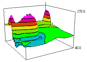
Iso lines: With this option, iso lines are plotted in a 3D-Plot as shown in the above image. The number and the colors of the iso lines must be given in the dialog „Scalar values“ respectively „Color definition“. The kind of visualization can be altered in the dialog „Visualize“ where following options can be given: Iso surfaces, Iso lines only, Angle of edges.

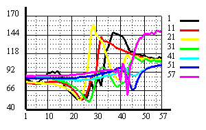
XZ-Plot: With this option an XY-Plot for selected lines of the matrix is done, as shown in the above image.

YZ-Plot: With this option a XY-Plot for selected columns of the matrix is done.

B L H: In the input field values for width, lengths and height of the 3D-Plot may be given. With XY-Plot, only values B and H are used.

ZMin ZMax: In the input field the smallest and the largest value to be used in z direction may be given.

Indices: For options „X lines“, „Y lines“, „XZ-Plot“ and “YZ-Plot” indices of individual lines respectively columns of the matrix that should be plotted may be given. A continuous sequence of indices may be given in the form i1,-i2,id where i1 is the smallest, i2 the largest index and id is an increment. For example 1,-61,10 means each 10^th index from 1 to 61. If the input field is empty, all lines respectively columns are plotted.

Color: In the input field color indices for the different curves may be given. If the field is empty, continuous indices are used, beginning by 1. For indices –1,-2,-3,... different line types are used.

Plot

Clicking this button a new graphics is done.

Switch Layer

Clicking this button, it can be switched between Array Plot and Structure plot, where only the corresponding OpenGL layers are switched on and off. This is done automatically, if a different property page of the dialog is used. If the dialog window is closed, the current array data is deleted and the used layer for the array plot is erased.

Plot vector fields

After giving the command Vector field a property dialog is popped up. This dialog remains active until it’s closed by „Cancel“.