Load post data: Load post processing data

It’s possible to load multiple data sets of the same or a different type.

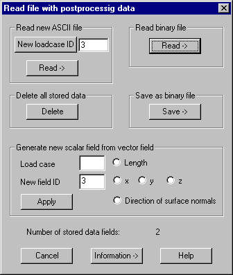
Following dialog shows the available options:

Read new text file

Read: After pressing this button a file selection box pops up to select the data filename to be read from.

New load case ID: Pressing this button, the next free load case ID will be set in the input field. If a load case ID > 0 is given, this will be used for the newly read data, else the load case ID will be taken from the first line of the file.

Delete all data in memory

Pressing button “Delete” all currently loaded data will be deleted.

Save as binary file

Pressing button “Save” all post processing data currently held in memory is saved to a binary file. The filename is selected from a file selection dialog. File extension will be .pos.

Read binary file

This button allows to loads a previously saved binary file.

Generate new scalar field from vector field

This option makes it possible to save the vector length or a single vector component from the vectors of a given vector field as a new scalar field.

Load case ID: The ID of the vector field to be translated to a scalar field must be given.

New field ID: This input field specifies the new load case ID for the generated scalar field. Next available ID is automatically set.

Length: With this option set the length of the vectors is used as scalar data.

x, y, z: This options select a vector component to be used as scalar data.

Direction of surface normals: This option uses the projection of the given vectors along the direction of the surface normal vectors of the elements as a scalar value.

Apply: After specifying the options this button does the calculation and saving of the scalar values.

Information

This button protocols all currently used data sets (load case, type, smallest and largest value) within a protocol window.

Plot scalar fields

After starting the command Scalar field a dialog with several property sheets pops up. This dialog remains active until it’s explicitly closed by „Cancel“. It can freely be switched between these sheets.

For the visualization of the distribution of the values of a given scalar field, elements with additional nodes on the edges (for example curved elements) and elements that have scalar values given in integration points are approximated by triangular surfaces. The number of such triangles is 32 with quadrilateral and 16 with triangular elements. Scalar values for the additional nodes used by this approximation are calculated by interpolation using all given scalar values on element nodes and integration points.